The p99 Tax: Why Your Database Benchmarks Are Lying to You

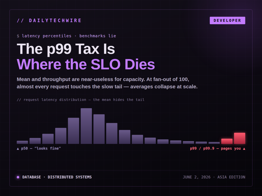
Most database benchmarks lead with throughput and a mean latency figure. Both are close to useless for capacity planning. The number that actually pages your on-call engineer is p99, and the gap between your p50 and your p99 is where every real infrastructure trade-off hides.

Why the tail matters more than the mean

A service that answers in 2ms at p50 and 400ms at p99 is not a 2ms service. If a single user request fans out to 20 backend calls, the probability that at least one call hits the p99 path is roughly 1 - 0.99^20, around 18%. At fan-out of 100, almost every user request touches a tail event. This is why averages collapse at scale: the more dependencies a request has, the more the slow tail dominates the experience.

p50 tells you what the system does when nothing is contending. p95 tells you what happens under normal load with some queuing. p99 and p99.9 tell you what happens when GC fires, a compaction kicks in, a connection pool saturates, or a noisy neighbor lands on the same host. Those are not edge cases at scale. They are the steady state.

Where the latency actually comes from

The tail is rarely one cause. Common contributors:

• GC pauses. Managed runtimes (JVM, Go, Node) introduce stop-the-world or concurrent collection costs. A GC pause that adds 30ms shows up almost entirely in p99, invisible at p50.
• Compaction and flushing. LSM-tree stores (RocksDB-backed engines, Cassandra, much of the time-series world) trade write amplification against read latency. Background compaction competes for disk I/O and CPU, and the spikes land on the tail.
• Connection pool saturation. When the pool is exhausted, requests queue. Queuing time is invisible until it isn't, and it shows up as a sudden p99 cliff rather than a gradual slope.
• Lock and contention. Row-level locks, B-tree page latches, and serialized writes to a hot key all serialize requests that would otherwise run concurrently.

The practical takeaway: a change that improves p50 often does nothing for, or actively worsens, p99. Adding a cache lowers the mean but can widen the tail, because cache misses now pay both the lookup cost and the origin cost.

The trade-offs nobody puts in the marketing

Replication and consistency. Strong consistency (quorum reads/writes) means a request waits for the slowest replica in the quorum. That slowest replica defines your tail. Relax to eventual consistency and p99 drops, but you accept stale reads. There is no configuration that gives you both low tail latency and strong consistency under partition.

Connection model. Per-request connections are simple and have a clean tail until you exhaust file descriptors. Pooling amortizes connection cost but introduces queuing under burst. The right pool size is workload-specific, and the default is almost always wrong for high-concurrency services.

Storage engine. B-tree engines (Postgres, MySQL/InnoDB) give predictable read latency and pay on writes. LSM engines absorb writes cheaply and pay unpredictably on reads during compaction. If your p99 read latency matters and your write volume is modest, the LSM advantage may cost you more than it saves.

Synchronous vs async commit. fsync on every commit protects durability and adds disk latency to every write tail. Group commit and async flush cut the tail but widen the window of data loss on crash. This is a durability-for-latency trade, and it should be a deliberate decision, not a default.

How to actually measure it

Three mistakes show up constantly:

1. Averaging percentiles across hosts. You cannot average p99s. The p99 of a fleet is not the mean of per-host p99s. Aggregate the raw histogram, then compute the percentile.
2. Coordinated omission. Most load generators that send a request, wait for the response, then send the next, systematically undercount the tail, because a slow response delays the next request that would have also been slow. Tools that maintain a fixed request schedule (the approach popularized by HdrHistogram and wrk2) avoid this. If your benchmark closes the loop, your p99 is optimistic.
3. Too-short test windows. Compaction, GC, and backup jobs run on their own schedules. A 60-second benchmark can miss every one of them and report a p99 you will never see in production.

What this means for capacity decisions

If you size capacity off p50, you will under-provision and your SLO will fail under load. The honest approach is to define the SLO at the percentile that matters (usually p99 or p99.9), measure with a non-coordinated-omission load profile over a window long enough to capture background work, and then decide which trade-off you are buying.

Lower tail latency is always available. It costs money (more replicas, more headroom), durability (async commit), consistency (relaxed reads), or complexity (sharding the hot key). The job is to pick which one to spend, not to pretend the tail isn't there.